Weighted Statistics
Introduction
There are several different reasons why a statistical analysis needs to adjust for weighting. In literature reasons are mainly diveded in to groups.The first group is when some of the measurements are known to be more precise than others. The more precise a measurement is, the larger weight it is given. The simplest case is when the weight are given before the measurements and they can be treated as deterministic. It becomes more complicated when the weight can be determined not until afterwards, and even more complicated if the weight depends on the value of the observable.
The second group of situations is when calculating averages over one distribution and sampling from another distribution. Compensating for this discrepency weights are introduced to the analysis. A simple example may be that we are interviewing people but for economical reasons we choose to interview more people from the city than from the countryside. When summarizing the statistics the answers from the city are given a smaller weight. In this example we are choosing the proportions of people from countryside and people from city being intervied. Hence, we can determine the weights before and consider them to be deterministic. In other situations the proportions are not deterministic, but rather a result from the sampling and the weights must be treated as stochastic and only in rare situations the weights can be treated as independent of the observable.
Since there are various origins for a weight occuring in a statistical analysis, there are various ways to treat the weights and in general the analysis should be tailored to treat the weights correctly. We have not chosen one situation for our implementations, so see specific function documentation for what assumtions are made. Though, common for implementations are the following:
- Setting all weights to unity yields the same result as the non-weighted version.
- Rescaling the weights does not change any function.
- Setting a weight to zero is equivalent to removing the data point.
The last point implies that a data point with zero weight is ignored also when the value is NaN. An important case is when weights are binary (either 1 or 0). Then we get the same result using the weighted version as using the data with weight not equal to zero and the non-weighted version. Hence, using binary weights and the weighted version missing values can be treated in a proper way.
AveragerWeighted
Mean
For any situation the weight is always designed so the weighted mean is calculated as , which obviously fulfills the conditions above.
In the case of varying measurement error, it could be motivated that the weight shall be  . We assume measurement error to be Gaussian and the likelihood to get our measurements is
 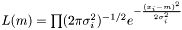 . We maximize the likelihood by taking the derivity with respect to
  on the logarithm of the likelihood
 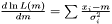 . Hence, the Maximum Likelihood method yields the estimator
  .
.
Variance
In case of varying variance, there is no point estimating a variance since it is different for each data point.
Instead we look at the case when we want to estimate the variance over  but are sampling from
  . For the mean of an observable
  we have
 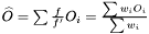 . Hence, an estimator of the variance of
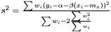
  is
is

This estimator fulfills that it is invariant under a rescaling and having a weight equal to zero is equivalent to removing the data point. Having all weights equal to unity we get  , which is the same as returned from Averager. Hence, this estimator is slightly biased, but still very efficient.
Standard Error
The standard error squared is equal to the expexted squared error of the estimation of . The squared error consists of two parts, the variance of the estimator and the squared bias:

 .
.
In the case when weights are included in analysis due to varying measurement errors and the weights can be treated as deterministic, we have


where we need to estimate  . Again we have the likelihood
 and taking the derivity with respect to
  ,
,

which yields an estimator  . This estimator is not ignoring weights equal to zero, because deviation is most often smaller than the expected infinity. Therefore, we modify the expression as follows
  and we get the following estimator of the variance of the mean
 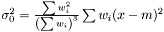 . This estimator fulfills the conditions above: adding a weight zero does not change it: rescaling the weights does not change it, and setting all weights to unity yields the same expression as in the non-weighted case.
In a case when it is not a good approximation to treat the weights as deterministic, there are two ways to get a better estimation. The first one is to linearize the expression  . The second method when the situation is more complicated is to estimate the standard error using a bootstrapping method.
AveragerPairWeighted
Here data points come in pairs (x,y). We are sampling from but want to measure from
  . To compensate for this decrepency, averages of
  are taken as
  . Even though,
  and
and  are not independent
  we assume that we can factorize the ratio and get
Covariance
Following the variance calculations for AveragerWeighted we have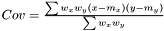 where
where 
Correlation
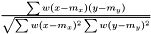
As the mean is estimated as , the variance is estimated as
 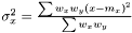 . As in the non-weighted case we define the correlation to be the ratio between the covariance and geometrical average of the variances
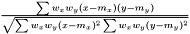 .
.
This expression fulfills the following
- Having N equal weights the expression reduces to the non-weighted expression.
- Adding a pair of data, in which one weight is zero is equivalent to ignoring the data pair.
- Correlation is equal to unity if and only if
 is equal to
  . Otherwise the correlation is between -1 and 1.
Score
Pearson
 .
.See AveragerPairWeighted correlation.
ROC
An interpretation of the ROC curve area is the probability that if we take one sample from class and one sample from class
  , what is the probability that the sample from class has greater value. The ROC curve area calculates the ratio of pairs fulfilling this

An geometrical interpretation is to have a number of squares where each square correspond to a pair of samples. The ROC curve follows the border between pairs in which the samples from class has a greater value and pairs in which this is not fulfilled. The ROC curve area is the area of those latter squares and a natural extension is to weight each pair with its two weights and consequently the weighted ROC curve area becomes
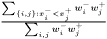
This expression is invariant under a rescaling of weight. Adding a data value with weight zero adds nothing to the exprssion, and having all weight equal to unity yields the non-weighted ROC curve area.
tScore
Assume that and originate from the same distribution  where
where  . We then estimate
  as
as 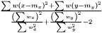 The variance of difference of the means becomes
 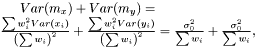 and consequently the t-score becomes
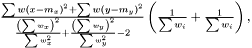
For a  we this expression get condensed down to
 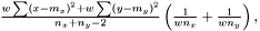 in other words the good old expression as for non-weighted.
FoldChange
Fold-Change is simply the difference between the weighted mean of the two groups
WilcoxonFoldChange
Taking all pair samples (one from class and one from class ) and calculating the weighted median of the distances.Distance
A Distance measures how far apart two ranges are. A Distance should preferably meet some criteria:
- It is symmetric,
 , that is distance from
  to
to  equals the distance from to .
 - Zero self-distance:

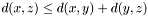
- Triangle inequality:
Weighted Distance
Weighted Distance is an extension of usual unweighted distances, in which each data point is accompanied with a weight. A weighted distance should meet some criteria:
- Having all unity weights should yield the unweighted case.
- Rescaling the weights,
 , does not change the distance.
 - Having a
 the distance should ignore corresponding , , and
  .
. - A zero weight should not result in a very different distance than a small weight, in other words, modifying a weight should change the distance in a continuous manner.
- The duplicate property. If data is coming in duplicate such that
 , then the case when
  should equal to if you set
  .
.
The last condition, duplicate property, implies that setting a weight to zero is not equivalent to removing the data point. This behavior is sensible because otherwise we would have a bias towards having ranges with small weights being close to other ranges. For a weighted distance, meeting these criteria, it might be difficult to show that the triangle inequality is fulfilled. For most algorithms the triangle inequality is not essential for the distance to work properly, so if you need to choose between fulfilling triangle inequality and these latter criteria it is preferable to meet the latter criteria.
In test/distance_test.cc there are tests for testing these properties.
Kernel
Polynomial Kernel
The polynomial kernel of degree is defined as
  , where
  is the linear kernel (usual scalar product). For the weighted case we define the linear kernel to be
 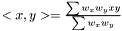 and the polynomial kernel can be calculated as before .
Gaussian Kernel
We define the weighted Gaussian kernel as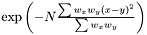 .
.Regression
Naive
Linear
We have the model
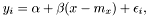
where  is the noise. The variance of the noise is inversely proportional to the weight,
  . In order to determine the model parameters, we minimimize the sum of quadratic errors.

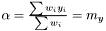
Taking the derivity with respect to  and
and  yields two conditions

and

or equivalently
and
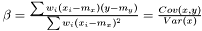
Note, by having all weights equal we get back the unweighted case. Furthermore, we calculate the variance of the estimators of and .
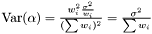
and 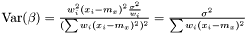
Finally, we estimate the level of noise,  . Inspired by the unweighted estimation
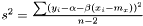
we suggest the following estimator