

Next: The Back-Propagation Family
Up: No Title
Previous: Introduction
When analyzing experimental data the standard procedure is to make various cuts
in observed kinematical variables  in order to single out desired
features. A specific selection of cuts corresponds to a particular set of feature
functions
  in terms of the
kinematical variables
  . This procedure is often not very systematic and
quite tedious. Ideally one would like to have an automated optimal choice of the
functions
  , which is exactly what feature recognition ANN aim at. For
a feed-forward ANN the following form of
  is often chosen

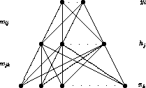
which corresponds to the architecture of fig.  . Here the ``weights''
 and
and  are the parameters to
be fitted to the data distributions and
  is the non-linear neuron
activation function, typically of the form

The bottom layer (input) in fig.  corresponds to sensor
variables
  and the
top layer to the (output) features
  (the feature functions
  ).
The hidden layer enables non-linear modeling of the sensor data.
Eq. (
 ) and fig.
  are easily generalized to more than
one hidden layer.
Using eq. ( ) for the output assumes that the output variables
represent classes and are of binary nature. The same architecture can
be used for real function mapping if
  are chosen linear, in which
case the outermost g is removed from the left hand side of (
 ).
).

Figure: A one hidden layer feed-forward neural network architecture.
The weights  and
and  are determined by minimizing
an error measure of the fit, e.g. a mean square error

between  and the desired feature values
  (targets) with respect
to the weights. In eq. (
 )
)  denotes patterns. For architectures
with non-linear hidden nodes no exact procedure exists for minimizing the
error and one has to rely on iterative methods, some of which are described
below.
Once the weights have been fitted to the data in this way, using labeled
data, the network should be able to model data it has never seen before.
The ability of the network to correctly model such unlabeled data is called
generalization performance.
When modeling data it is always crucial for the generalization performance
that the number of data points well exceeds the number of parameters (in our
case the number of weights  ). For a given set of sensor variables
this can be accomplished by
- Preprocessing using e.g. Principal Component Analysis.
- Building in a priori known symmetries into the problem --
``weight sharing''.
- Adding complexity terms to the error (eq. (
 )) to
regularize the network.
- Inspection of the final network to remove redundant parameters.
all of which we will return to later.


Next: The Back-Propagation Family
Up: No Title
Previous: Introduction
System PRIVILEGED Account
Fri Feb 24 11:28:59 MET 1995
 in order to single out desired
features. A specific selection of cuts corresponds to a particular set of feature
functions
  in terms of the
kinematical variables
  . This procedure is often not very systematic and
quite tedious. Ideally one would like to have an automated optimal choice of the
functions
  , which is exactly what feature recognition ANN aim at. For
a feed-forward ANN the following form of
  is often chosen

 and
and  are the parameters to
be fitted to the data distributions and
  is the non-linear neuron
activation function, typically of the form

 and the
top layer to the (output) features
  (the feature functions
  ).
The hidden layer enables non-linear modeling of the sensor data.
Eq. (
 are chosen linear, in which
case the outermost g is removed from the left hand side of (
 and
and  are determined by minimizing
an error measure of the fit, e.g. a mean square error

 and the desired feature values
  (targets) with respect
to the weights. In eq. (
 denotes patterns. For architectures
with non-linear hidden nodes no exact procedure exists for minimizing the
error and one has to rely on iterative methods, some of which are described
below.
 ). For a given set of sensor variables
this can be accomplished by